.ipynb .pdf

repository open issue

Binder Live Code

Contents

2022-04-22 Adaptivity

Last time

• Implicit and explicit methods

• Stiff equations

Today

• More on stiffness

• PDE examples

• Accuracy

• Adaptivity

• FCQ

using LinearAlgebra
using Plots
default(linewidth=4, legendfontsize=12)

struct RKTable
    A::Matrix
    b::Vector
    c::Vector
    function RKTable(A, b)
        s = length(b)
        A = reshape(A, s, s)
        c = vec(sum(A, dims=2))
        new(A, b, c)
    end
end

function rk_stability(z, rk)
    s = length(rk.b)
    1 + z * rk.b' * ((I - z*rk.A) \ ones(s))
end

rk4 = RKTable([0 0 0 0; .5 0 0 0; 0 .5 0 0; 0 0 1 0], [1, 2, 2, 1] / 6)
heun = RKTable([0 0; 1 0], [.5, .5])
Rz_theta(z, theta) = (1 + (1 - theta)*z) / (1 - theta*z)

function ode_rk_explicit(f, u0; tfinal=1, h=0.1, table=rk4)
    u = copy(u0)
    t = 0.
    n, s = length(u), length(table.c)
    fY = zeros(n, s)
    thist = [t]
    uhist = [u0]
    while t < tfinal
        tnext = min(t+h, tfinal)
        h = tnext - t
        for i in 1:s
            ti = t + h * table.c[i]
            Yi = u + h * sum(fY[:,1:i-1] * table.A[i,1:i-1], dims=2)
            fY[:,i] = f(ti, Yi)
        end
        u += h * fY * table.b
        t = tnext
        push!(thist, t)
        push!(uhist, u)
    end
    thist, hcat(uhist...)
end

function plot_stability(Rz, method; xlim=(-3, 2), ylim=(-1.5, 1.5))
    x = xlim[1]:.02:xlim[2]
    y = ylim[1]:.02:ylim[2]
    plot(title="Stability: $method", aspect_ratio=:equal, xlim=xlim, ylim=ylim)
    heatmap!(x, y, (x, y) -> abs(Rz(x + 1im*y)), c=:bwr, clims=(0, 2))
    contour!(x, y, (x, y) -> abs(Rz(x + 1im*y)), color=:black, linewidth=2, levels=[1.])
    plot!(x->0, color=:black, linewidth=1, label=:none)
    plot!([0, 0], [ylim...], color=:black, linewidth=1, label=:none)
end

plot_stability (generic function with 1 method)

The \(\theta\) method

Forward and backward Euler are bookends of the family known as \(\theta\) methods.

\[ \tilde u(h) = u(0) + h f\Big(\theta h, \theta\tilde u(h) + (1-\theta)u(0) \Big) \]

which, for linear problems, is solved as

\[ (I - h \theta A) u(h) = \Big(I + h (1-\theta) A \Big) u(0) . \]

\(\theta=0\) is explicit Euler, \(\theta=1\) is implicit Euler, and \(\theta=1/2\) are the midpoint or trapezoid rules (equivalent for linear problems). The stability function is

\[ R(z) = \frac{1 + (1-\theta)z}{1 - \theta z}. \]

Rz_theta(z, theta) = (1 + (1-theta)*z) / (1 - theta*z)
theta = .6
plot_stability(z -> Rz_theta(z, theta), "\$\\theta=$theta\$", 
    xlim=(-20, 1))

\(\theta\) method for the oscillator

function ode_theta_linear(A, u0; forcing=zero, tfinal=1, h=0.1, theta=.5)
    u = copy(u0)
    t = 0.
    thist = [t]
    uhist = [u0]
    while t < tfinal
        tnext = min(t+h, tfinal)
        h = tnext - t
        rhs = (I + h*(1-theta)*A) * u .+ h*forcing(t+h*theta)
        u = (I - h*theta*A) \ rhs
        t = tnext
        push!(thist, t)
        push!(uhist, u)
    end
    thist, hcat(uhist...)
end

ode_theta_linear (generic function with 1 method)

# Test on oscillator
A = [0 1; -1 0]
theta = 1
thist, uhist = ode_theta_linear(A, [0., 1], h=.2, theta=theta, tfinal=20)
scatter(thist, uhist')
plot!([cos, sin])

\(\theta\) method for the cosine decay

k = 50
theta = .5
thist, uhist = ode_theta_linear(-k, [.2], forcing=t -> k*cos(t), tfinal=5, h=.5, theta=theta)
scatter(thist, uhist[1,:], title="\$\\theta = $theta\$")
plot!(cos, size=(800, 500))

Stability classes and the \(\theta\) method

Definition: \(A\)-stability

A method is \(A\)-stable if the stability region

\[ \{ z : |R(z)| \le 1 \} \]

contains the entire left half plane

\[ \Re[z] \le 0 .\]

This means that the method can take arbitrarily large time steps without becoming unstable (diverging) for any problem that is indeed physically stable.

Definition: \(L\)-stability

A time integrator with stability function \(R(z)\) is \(L\)-stable if

\[ \lim_{z\to\infty} R(z) = 0 .\]

For the \(\theta\) method, we have

\[ \lim_{z\to \infty} \frac{1 + (1-\theta)z}{1 - \theta z} = \frac{1-\theta}{\theta} . \]

Evidently only \(\theta=1\) is \(L\)-stable.

Heat equation as linear ODE

• How do different \(\theta \in [0, 1]\) compare in terms of stability?

• Are there artifacts even when the solution is stable?

using SparseArrays

function heat_matrix(n)
    dx = 2 / n
    rows = [1]
    cols = [1]
    vals = [0.]
    wrap(j) = (j + n - 1) % n + 1
    for i in 1:n
        append!(rows, [i, i, i])
        append!(cols, wrap.([i-1, i, i+1]))
        append!(vals, [1, -2, 1] ./ dx^2)
    end
    sparse(rows, cols, vals)
end
heat_matrix(5)

5×5 SparseMatrixCSC{Float64, Int64} with 15 stored entries:
 -12.5     6.25     ⋅       ⋅      6.25
   6.25  -12.5     6.25     ⋅       ⋅ 
    ⋅      6.25  -12.5     6.25     ⋅ 
    ⋅       ⋅      6.25  -12.5     6.25
   6.25     ⋅       ⋅      6.25  -12.5

n = 200
A = heat_matrix(n)
x = LinRange(-1, 1, n+1)[1:end-1]
u0 = exp.(-200 * x .^ 2)
@time thist, uhist = ode_theta_linear(A, u0, h=.1, theta=1, tfinal=1);
nsteps = size(uhist, 2)
plot(x, uhist[:, 1:5])

  1.281199 seconds (4.38 M allocations: 230.188 MiB, 7.18% gc time, 99.80% compilation time)

Advection as a linear ODE

function advect_matrix(n; upwind=false)
    dx = 2 / n
    rows = [1]
    cols = [1]
    vals = [0.]
    wrap(j) = (j + n - 1) % n + 1
    for i in 1:n
        append!(rows, [i, i])
        if upwind
            append!(cols, wrap.([i-1, i]))
            append!(vals, [1., -1] ./ dx)
        else
            append!(cols, wrap.([i-1, i+1]))
            append!(vals, [1., -1] ./ 2dx)
        end
    end
    sparse(rows, cols, vals)
end
advect_matrix(5)

5×5 SparseMatrixCSC{Float64, Int64} with 11 stored entries:
  0.0   -1.25    ⋅      ⋅     1.25
  1.25    ⋅    -1.25    ⋅      ⋅ 
   ⋅     1.25    ⋅    -1.25    ⋅ 
   ⋅      ⋅     1.25    ⋅    -1.25
 -1.25    ⋅      ⋅     1.25    ⋅ 

n = 50
A = advect_matrix(n, upwind=false)
x = LinRange(-1, 1, n+1)[1:end-1]
u0 = exp.(-9 * x .^ 2)
@time thist, uhist = ode_theta_linear(A, u0, h=.04, theta=1, tfinal=1.);
nsteps = size(uhist, 2)
plot(x, uhist[:, 1:(nsteps÷8):end])

  0.061281 seconds (167.05 k allocations: 10.873 MiB, 96.58% compilation time)

Spectrum of operators

theta=.5
h = .1
plot_stability(z -> Rz_theta(z, theta), "\$\\theta=$theta, h=$h\$")
ev = eigvals(Matrix(h*advect_matrix(20, upwind=true)))
scatter!(real(ev), imag(ev))

theta=.5
h = .2 / 4
plot_stability(z -> Rz_theta(z, theta), "\$\\theta=$theta, h=$h\$")
ev = eigvals(Matrix(h*heat_matrix(20)))
scatter!(real(ev), imag(ev))

Stiffness

Stiff equations are problems for which explicit methods don’t work. (Hairer and Wanner, 2002)

• “stiff” dates to Curtiss and Hirschfelder (1952)

We’ll use the cosine relaxation example \(y_t = -k(y - \cos t)\) using the \(\theta\) method, varying \(k\) and \(\theta\).

function ode_error(h; theta=.5, k=10)
    u0 = [.2]
    thist, uhist = ode_theta_linear(-k, u0, forcing=t -> k*cos(t), tfinal=3, h=h, theta=theta)
    T = thist[end]
    u_exact = (u0 .- k^2/(k^2+1)) * exp(-k*T) .+ k*(sin(T) + k*cos(T))/(k^2 + 1)
    uhist[1,end] .- u_exact
end

ode_error (generic function with 1 method)

hs = .5 .^ (1:8)
errors = ode_error.(hs, theta=0, k=5)
plot(hs, norm.(errors), marker=:auto, xscale=:log10, yscale=:log10)
plot!(hs, hs, label="\$h\$", legend=:topleft)
plot!(hs, hs.^2, label="\$h^2\$", ylabel="cost", xlabel="\$\\Delta t\$")

Examples of ODE systems

Stiff problems posess multiple time scales and the fastest scale is “not interesting”

Stiff

• The ocean

Non-stiff

• The ocean

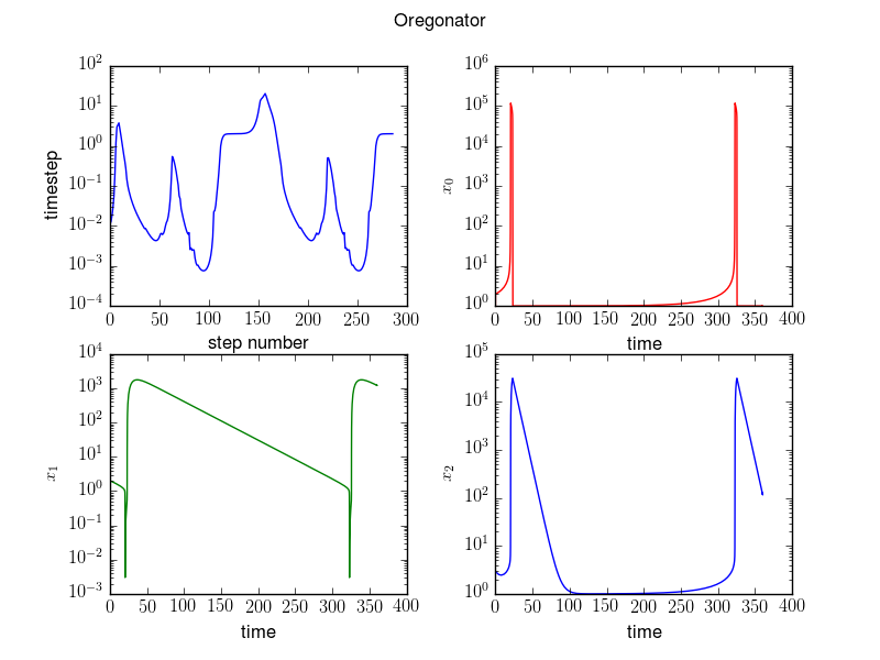
Adaptive time integrators

The Oregonator mechanism in chemical kinetics describes an oscillatory chemical system. It consists of three species with concentrations \(\mathbf x = [x_0,x_1,x_2]^T\) (scaled units) and the evolution equations

\[\begin{split} \mathbf {x'} = \begin{bmatrix} 77.27 \big(x_1 + x_0 (1 - 8.375\cdot 10^{-6} x_0 - x_1) \big) \\ \frac{1}{77.27} \big(x_2 - (1 + x_0) x_1 \big) \\ 0.161 (x_0 - x_2) \end{bmatrix} . \end{split}\]

We simulate from the initial conditions \(\mathbf x_0 = [1, 2, 3]^T\).

Plan for next week

Monday

• I will answer questions/work problems on Monday.

• Please chat with your neighbor and suggest ideas in Zulip.

Wednesday

• Groups will present 5-minute lightning talks on Wednesday.

• If you prefer to pre-record, do that and share a link on Zulip.

• If you have a group, but it hasn’t been mentioned on Zulip, please identify yourself so I can check in (scheduling and format).

previous

2022-04-20 Stiff equations