
2022-01-24 Convergence classes
Contents
2022-01-24 Convergence classes
Office hours: Monday 9-10pm, Tuesday 2-3pm, Thursday 2-3pm
This week will stay virtual. Plan is to start in-person the following Monday (Jan 31)
Last time
Forward and backward error
Computing volume of a polygon
Rootfinding examples
Use Roots.jl to solve
Introduce Bisection
Today
Discuss rootfinding as a modeling tool
Limitations of bisection
Convergence classes
Intro to Newton methods
using Plots
default(linewidth=4)
Stability demo: Volume of a polygon
X = ([1 0; 2 1; 1 3; 0 1; -1 1.5; -2 -1; .5 -2; 1 0])
R(θ) = [cos(θ) -sin(θ); sin(θ) cos(θ)]
Y = X * R(deg2rad(10))' .+ [1e4 1e4]
plot(Y[:,1], Y[:,2], seriestype=:shape, aspect_ratio=:equal)

using LinearAlgebra
function pvolume(X)
    n = size(X, 1)
    vol = sum(det(X[i:i+1, :]) / 2 for i in 1:n-1)
end

@show pvolume(Y)
[det(Y[i:i+1, :]) for i in 1:size(Y, 1)-1]
A = Y[2:3, :]
sum([A[1,1] * A[2,2], - A[1,2] * A[2,1]])
X
pvolume(Y) = 9.249999989226126
8×2 Matrix{Float64}:
  1.0   0.0
  2.0   1.0
  1.0   3.0
  0.0   1.0
 -1.0   1.5
 -2.0  -1.0
  0.5  -2.0
  1.0   0.0
Why don’t we even get the first digit correct? These numbers are only \(10^8\) and \(\epsilon_{\text{machine}} \approx 10^{-16}\) so shouldn’t we get about 8 digits correct?
Rootfinding
Given \(f(x)\), find \(x\) such that \(f(x) = 0\).
We’ll work with scalars (\(f\) and \(x\) are just numbers) for now, and revisit later when they vector-valued.
Change inputs to outputs
\(f(x; b) = x^2 - b\)
\(x(b) = \sqrt{b}\)
\(f(x; b) = \tan x - b\)
\(x(b) = \arctan b\)
\(f(x) = \cos x + x - b\)
\(x(b) = ?\)
We aren’t given \(f(x)\), but rather an algorithm f(x) that approximates it.
Sometimes we get extra information, like
fp(x)that approximates \(f'(x)\)If we have source code for
f(x), maybe it can be transformed “automatically”
Nesting matryoshka dolls of rootfinding
I have a function (pressure, temperature) \(\mapsto\) (density, energy)
I need (density, energy) \(\mapsto\) (pressure, temperature)
I know what condition is satisfied across waves, but not the state on each side.
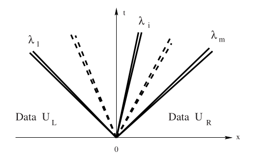
Given a proposed state, I can measure how much (mass, momentum, energy) is not conserved.
Find the solution that conserves exactly
I can compute lift given speed and angle of attack
How much can the plane lift?
How much can it lift on a short runway?
Discuss: rootfinding and inverse problems
Inverse kinematics for robotics
(statics) how much does each joint an robotic arm need to move to grasp an object
(with momentum) fastest way to get there (motors and arms have finite strength)
similar for virtual reality
Infer a light source (or lenses/mirrors) from an iluminated scene
Imaging
radiologist seeing an x-ray is mentally inferring 3D geometry from 2D image
computed tomography (CT) reconstructs 3D model from multiple 2D x-ray images
seismology infers subsurface/deep earth structure from seismograpms
Iterative bisection
f(x) = cos(x) - x
hasroot(f, a, b) = f(a) * f(b) < 0
function bisect_iter(f, a, b, tol)
    hist = Float64[]
    while abs(b - a) > tol
        mid = (a + b) / 2
        push!(hist, mid)
        if hasroot(f, a, mid)
            b = mid
        else
            a = mid
        end
    end
    hist
end
bisect_iter (generic function with 1 method)
length(bisect_iter(f, -1, 3, 1e-20))
56
Let’s plot the error
where \(r\) is the true root, \(f(r) = 0\).
hist = bisect_iter(f, -1, 3, 1e-10)
r = hist[end] # What are we trusting?
hist = hist[1:end-1]
scatter( abs.(hist .- r), yscale=:log10)
ks = 1:length(hist)
plot!(ks, 4 * (.5 .^ ks))

Evidently the error \(e_k = x_k - x_*\) after \(k\) bisections satisfies the bound
Convergence classes
A convergent rootfinding algorithm produces a sequence of approximations \(x_k\) such that
ρ = 0.8
errors = [1.]
for i in 1:30
    next_e = errors[end] * ρ
    push!(errors, next_e)
end
plot(errors, yscale=:log10, ylims=(1e-10, 1))

e = hist .- r
scatter(abs.(errors[2:end] ./ errors[1:end-1]), ylims=(0,1))

Bisection: A = q-linearly convergent, B = r-linearly convergent, C = neither
Remarks on bisection
Specifying an interval is often inconvenient
An interval in which the function changes sign guarantees convergence (robustness)
No derivative information is required
If bisection works for \(f(x)\), then it works and gives the same accuracy for \(f(x) \sigma(x)\) where \(\sigma(x) > 0\).
Roots of even degree are problematic
A bound on the solution error is directly available
The convergence rate is modest – one iteration per bit of accuracy
Newton-Raphson Method
Much of numerical analysis reduces to Taylor series, the approximation
In numerical computation, it is exceedingly rare to look beyond the first-order approximation
An implementation
function newton(f, fp, x0; tol=1e-8, verbose=false)
    x = x0
    for k in 1:100 # max number of iterations
        fx = f(x)
        fpx = fp(x)
        if verbose
            println("[$k] x=$x  f(x)=$fx  f'(x)=$fpx")
        end
        if abs(fx) < tol
            return x, fx, k
        end
        x = x - fx / fpx
    end
end

f(x) = cos(x) - x
fp(x) = -sin(x) - 1
newton(f, fp, 1; tol=1e-15, verbose=true)
[1] x=1  f(x)=-0.45969769413186023  f'(x)=-1.8414709848078965
[2] x=0.7503638678402439  f(x)=-0.018923073822117442  f'(x)=-1.6819049529414878
[3] x=0.7391128909113617  f(x)=-4.6455898990771516e-5  f'(x)=-1.6736325442243012
[4] x=0.739085133385284  f(x)=-2.847205804457076e-10  f'(x)=-1.6736120293089505
[5] x=0.7390851332151607  f(x)=0.0  f'(x)=-1.6736120291832148
(0.7390851332151607, 0.0, 5)