2022-02-14 QR Factorization

2022-02-14 QR Factorization¶

Sahitya’s office hours: Friday 11-12:30

Last time¶

Revisit projections, rotations, and reflections
Constructing orthogonal bases

Today¶

Gram-Schmidt process
QR factorization
Stability and ill conditioning
Intro to performance modeling

using LinearAlgebra
using Plots
using Polynomials
default(linewidth=4, legendfontsize=12)

function vander(x, k=nothing)
    if isnothing(k)
        k = length(x)
    end
    m = length(x)
    V = ones(m, k)
    for j in 2:k
        V[:, j] = V[:, j-1] .* x
    end
    V
end

vander (generic function with 2 methods)

Gram-Schmidt orthogonalization¶

Suppose we’re given some vectors and want to find an orthogonal basis for their span.

\[\begin{split} \Bigg[ a_1 \Bigg| a_2 \Bigg] = \Bigg[ q_1 \Bigg| q_2 \Bigg] \begin{bmatrix} r_{11} & r_{12} \\ 0 & r_{22} \end{bmatrix} \end{split}\]

A naive algorithm¶

function gram_schmidt_naive(A)
    m, n = size(A)
    Q = zeros(m, n)
    R = zeros(n, n)
    for j in 1:n
        v = A[:,j]
        for k in 1:j-1
            r = Q[:,k]' * v
            v -= Q[:,k] * r
            R[k,j] = r
        end
        R[j,j] = norm(v)
        Q[:,j] = v / R[j,j]
    end
    Q, R
end

gram_schmidt_naive (generic function with 1 method)

x = LinRange(-1, 1, 10)
A = vander(x, 4)
Q, R = gram_schmidt_naive(A)
@show norm(Q' * Q - I)
@show norm(Q * R - A);

norm(Q' * Q - I) = 3.684346652564232e-16
norm(Q * R - A) = 1.6779947319649215e-16

What do orthogonal polynomials look like?¶

x = LinRange(-1, 1, 200)
A = vander(x, 6)
Q, R = gram_schmidt_naive(A)
plot(x, Q)

../_images/2022-02-14-qr-factorization_7_0.svg

What happens if we use more than 50 values of \(x\)? Is there a continuous limit?

Theorem¶

Every full-rank \(m\times n\) matrix (\(m \ge n\)) has a unique reduced \(Q R\) factorization with \(R_{j,j} > 0\)¶

The algorithm we’re using generates this matrix due to the line:

        R[j,j] = norm(v)

Solving equations using \(QR = A\)¶

If \(A x = b\) then \(Rx = Q^T b\).

x1 = [-0.9, 0.1, 0.5, 0.8] # points where we know values
y1 = [1, 2.4, -0.2, 1.3]
scatter(x1, y1)
A = vander(x1, 3)
Q, R = gram_schmidt_naive(A)
p = R \ (Q' * y1)
p = A \ y1
plot!(x, vander(x, 3) * p)

../_images/2022-02-14-qr-factorization_11_0.svg

How accurate is it?¶

m = 30
x = LinRange(-1, 1, m)
A = vander(x, m)
Q, R = gram_schmidt_naive(A)
@show norm(Q' * Q - I)
@show norm(Q * R - A)

norm(Q' * Q - I) = 0.00043830040698919693
norm(Q * R - A) = 1.25091691161899e-15

1.25091691161899e-15

A variant with more parallelism¶

(9)¶\[\begin{align} (I - q_2 q_2^T) (I - q_1 q_1^T) v &= (I - q_1 q_1^T - q_2 q_2^T + q_2 q_2^T q_1 q_1^T) v \\ &= \Bigg( I - \Big[ q_1 \Big| q_2 \Big] \begin{bmatrix} q_1^T \\ q_2^T \end{bmatrix} \Bigg) v \end{align}\]

function gram_schmidt_classical(A)
    m, n = size(A)
    Q = zeros(m, n)
    R = zeros(n, n)
    for j in 1:n
        v = A[:,j]
        R[1:j-1,j] = Q[:,1:j-1]' * v
        v -= Q[:,1:j-1] * R[1:j-1,j]
        R[j,j] = norm(v)
        Q[:,j] = v / norm(v)
    end
    Q, R
end

gram_schmidt_classical (generic function with 1 method)

m = 10
x = LinRange(-1, 1, m)
A = vander(x, m)
Q, R = gram_schmidt_classical(A)
@show norm(Q' * Q - I)
@show norm(Q * R - A)

norm(Q' * Q - I) = 6.339875256299394e-11
norm(Q * R - A) = 1.217027619812654e-16

1.217027619812654e-16

Cost of Gram-Schmidt?¶

We’ll count flops (addition, multiplication, division*)
Inner product \(\sum_{i=1}^m x_i y_i\)?
Vector “axpy”: \(y_i = a x_i + y_i\), \(i \in [1, 2, \dotsc, m]\).
Look at the inner loop:

for k in 1:j-1
    r = Q[:,k]' * v
    v -= Q[:,k] * r
    R[k,j] = r
end

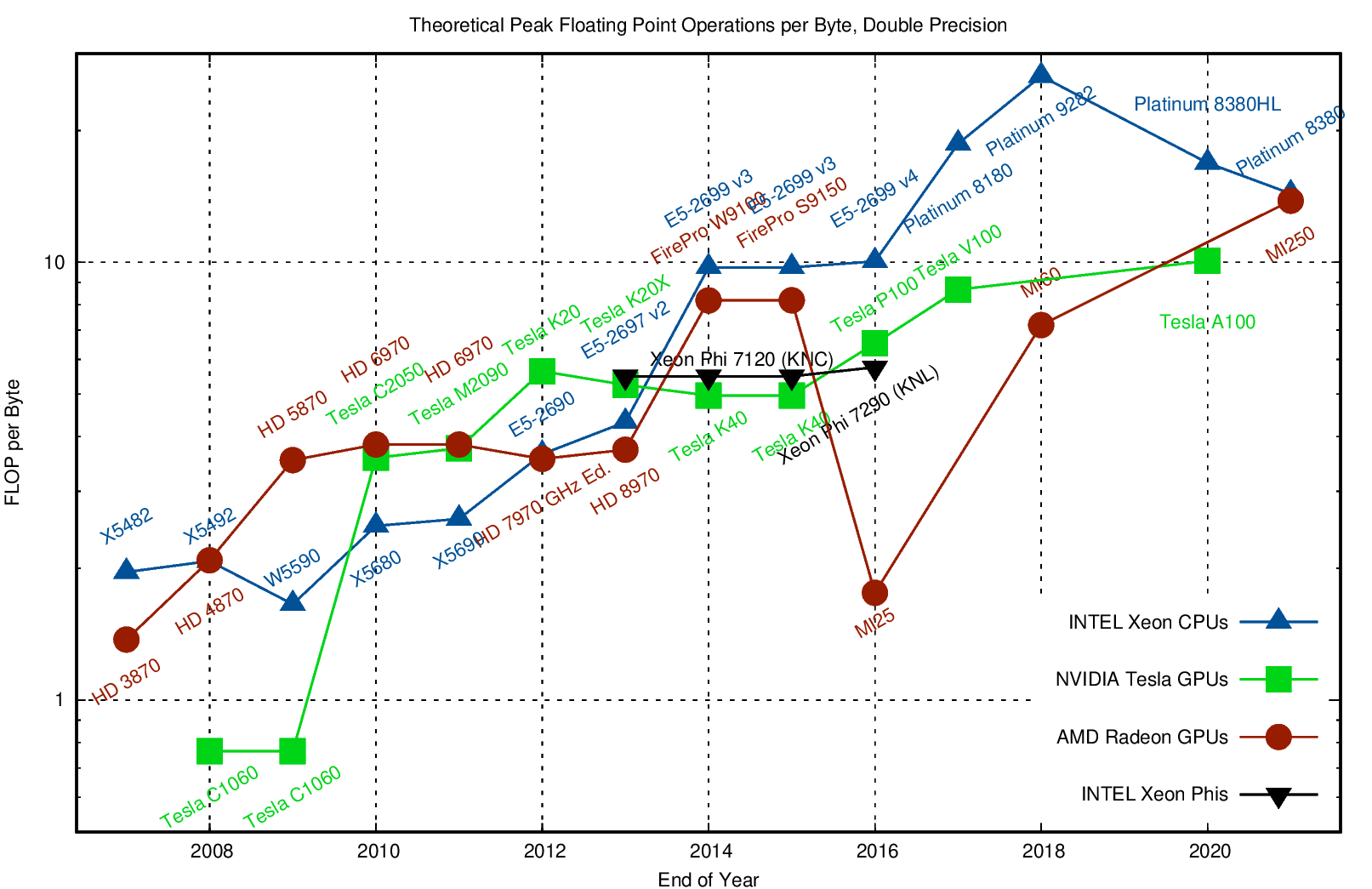
Counting flops is a bad model¶

We load a single entry (8 bytes) and do 2 flops (add + multiply). That’s an arithmetic intensity of 0.25 flops/byte.
Current hardware can do about 10 flops per byte, so our best algorithms will run at about 2% efficiency.
Need to focus on memory bandwidth, not flops.

Dense matrix-matrix mulitply¶

2022-02-11 Gram-Schmidt

2022-02-16 QR Stability

Numerical Computation