
2022-02-18 Householder QR
Contents
2022-02-18 Householder QR
Last time
Stability and ill conditioning
Intro to performance modeling
Classical vs Modified Gram-Schmidt
Today
Performance strategies
Right vs left-looking algorithms
Elementary reflectors
Householder QR
using LinearAlgebra
using Plots
using Polynomials
default(linewidth=4, legendfontsize=12)

function vander(x, k=nothing)
    if isnothing(k)
        k = length(x)
    end
    m = length(x)
    V = ones(m, k)
    for j in 2:k
        V[:, j] = V[:, j-1] .* x
    end
    V
end
vander (generic function with 2 methods)
A Gram-Schmidt with more parallelism
function gram_schmidt_classical(A)
    m, n = size(A)
    Q = zeros(m, n)
    R = zeros(n, n)
    for j in 1:n
        v = A[:,j]
        R[1:j-1,j] = Q[:,1:j-1]' * v
        v -= Q[:,1:j-1] * R[1:j-1,j]
        R[j,j] = norm(v)
        Q[:,j] = v / R[j,j]
    end
    Q, R
end
gram_schmidt_classical (generic function with 1 method)
m = 20
x = LinRange(-1, 1, m)
A = vander(x, m)
Q, R = gram_schmidt_classical(A)
@show norm(Q' * Q - I)
@show norm(Q * R - A)
norm(Q' * Q - I) = 1.4985231287367549
norm(Q * R - A) = 7.350692433565389e-16
7.350692433565389e-16
Why does order of operations matter?
is not exact in finite arithmetic.
We can look at the size of what’s left over
We project out the components of our vectors in the directions of each \(q_j\).
x = LinRange(-1, 1, 20)
A = vander(x)
Q, R = gram_schmidt_classical(A)
scatter(diag(R), yscale=:log10)

The next vector is almost linearly dependent
x = LinRange(-1, 1, 20)
A = vander(x)
Q, _ = gram_schmidt_classical(A)
#Q, _ = qr(A)
v = A[:,end]
@show norm(v)
scatter(abs.(Q[:,1:end-1]' * v), yscale=:log10)
norm(v) = 1.4245900685395503

Cost of Gram-Schmidt?
We’ll count flops (addition, multiplication, division*)
Inner product \(\sum_{i=1}^m x_i y_i\)?
Vector “axpy”: \(y_i = a x_i + y_i\), \(i \in [1, 2, \dotsc, m]\).
Look at the inner loop:
for k in 1:j-1
    r = Q[:,k]' * v
    v -= Q[:,k] * r
    R[k,j] = r
end
Counting flops is a bad model
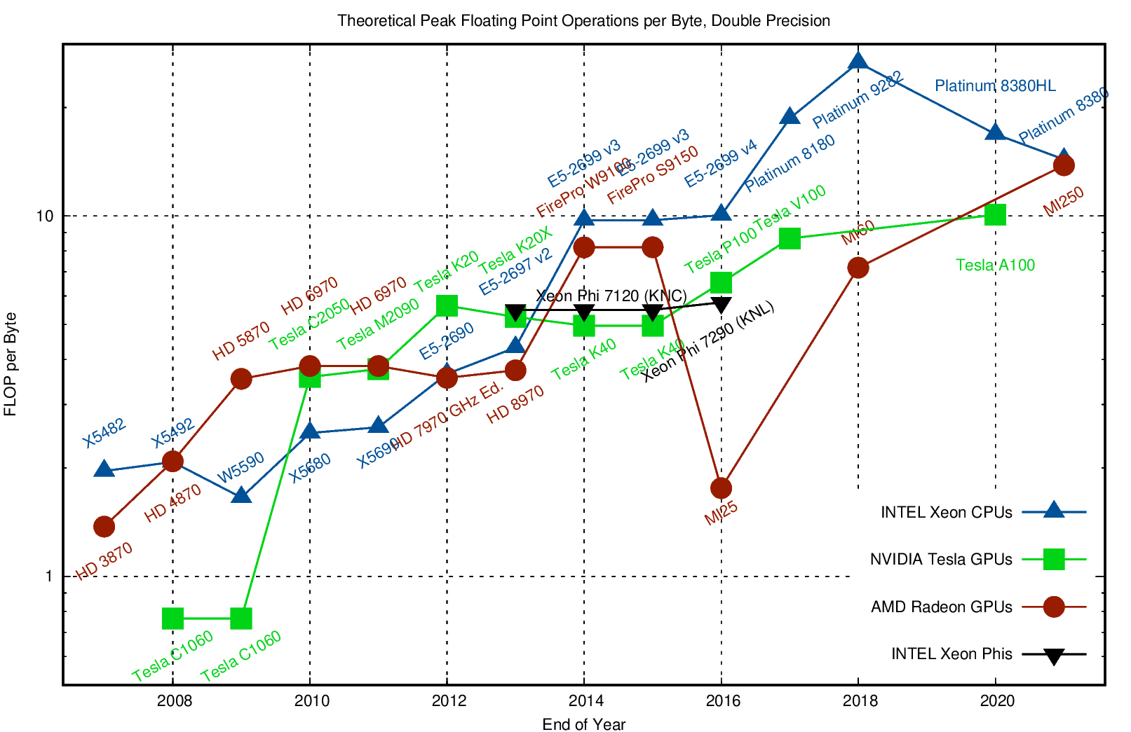
We load a single entry (8 bytes) and do 2 flops (add + multiply). That’s an arithmetic intensity of 0.25 flops/byte.
Current hardware can do about 10 flops per byte, so our best algorithms will run at about 2% efficiency.
Need to focus on memory bandwidth, not flops.
Inherent data dependencies
Right-looking modified Gram-Schmidt
function gram_schmidt_modified(A)
    m, n = size(A)
    Q = copy(A)
    R = zeros(n, n)
    for j in 1:n
        R[j,j] = norm(Q[:,j])
        Q[:,j] /= R[j,j]
        R[j,j+1:end] = Q[:,j]'*Q[:,j+1:end]
        Q[:,j+1:end] -= Q[:,j]*R[j,j+1:end]'
    end
    Q, R
end
gram_schmidt_modified (generic function with 1 method)
m = 20
x = LinRange(-1, 1, m)
A = vander(x, m)
Q, R = gram_schmidt_modified(A)
@show norm(Q' * Q - I)
@show norm(Q * R - A)
norm(Q' * Q - I) = 8.486718528276085e-9
norm(Q * R - A) = 8.709998074379606e-16
8.709998074379606e-16
Classical versus modified?
Classical
Really unstable, orthogonality error of size \(1 \gg \epsilon_{\text{machine}}\)
Don’t need to know all the vectors in advance
Modified
Needs to be right-looking for efficiency
Less unstable, but orthogonality error \(10^{-9} \gg \epsilon_{\text{machine}}\)
m = 20
x = LinRange(-1, 1, m)
A = vander(x, m)
Q, R = qr(A)
@show norm(Q' * Q - I)
norm(Q' * Q - I) = 3.1195004131362406e-15
3.1195004131362406e-15
Householder QR
Gram-Schmidt constructed a triangular matrix \(R\) to orthogonalize \(A\) into \(Q\). Each step was a projector, which is a rank-deficient operation. Householder uses orthogonal transformations (reflectors) to triangularize.
The structure of the algorithm is
Constructing the \(Q_j\)
Each of our \(Q_j\) will have the form
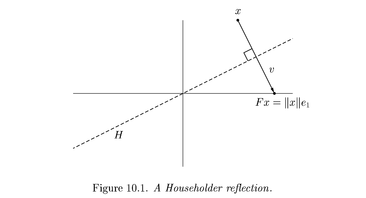
The reflection, as depicted above by Trefethen and Bau (1999) can be written \(F = I - 2 \frac{v v^T}{v^T v}\).
Adventures in reflection
A = rand(4, 4); A += A'
v = copy(A[:,1])
v[1] -= norm(v)
v = normalize(v)
F = I - 2 * v * v'
B = F * A
4×4 Matrix{Float64}:
  2.1741       1.25714    0.99767    1.18672
 -6.55398e-16  0.118113   0.765884   1.28508
 -2.96172e-16  1.05277   -0.0743418  0.52617
 -8.46837e-16  0.985914   0.0179292  0.779973
v = copy(B[2:end, 2])
v[1] -= norm(v); v = normalize(v)
F = I - 2 * v * v'
B[2:end, 2:end] = F * B[2:end, 2:end]
B
4×4 Matrix{Float64}:
  2.1741       1.25714      0.99767   1.18672
 -6.55398e-16  1.44717      0.020642  1.01903
 -2.96172e-16  0.0          0.515979  0.736919
 -8.46837e-16  1.11022e-16  0.570759  0.977337
An algorithm
function qr_householder_naive(A)
    m, n = size(A)
    R = copy(A)
    V = [] # list of reflectors
    for j in 1:n
        v = copy(R[j:end, j])
        v[1] -= norm(v)
        v = normalize(v)
        R[j:end,j:end] -= 2 * v * (v' * R[j:end,j:end])
        push!(V, v)
    end
    V, R
end
qr_householder_naive (generic function with 1 method)
m = 4
x = LinRange(-1, 1, m)
A = vander(x, m)
V, R = qr_householder_naive(A)
_, R_ = qr(A)
R_
4×4 Matrix{Float64}:
 -2.0  0.0      -1.11111      0.0
  0.0  1.49071   1.38778e-17  1.3582
  0.0  0.0       0.888889     9.71445e-17
  0.0  0.0       0.0          0.397523
How to interpret \(V\) as \(Q\)?
function reflectors_mult(V, x)
    y = copy(x)
    for v in reverse(V)
        n = length(v) - 1
        y[end-n:end] -= 2 * v * (v' * y[end-n:end])
    end
    y
end

function reflectors_to_dense(V)
    m = length(V[1])
    Q = diagm(ones(m))
    for j in 1:m
        Q[:,j] = reflectors_mult(V, Q[:,j])
    end
    Q
end
reflectors_to_dense (generic function with 1 method)
m = 20
x = LinRange(-1, 1, m)
A = vander(x, m)
V, R = qr_householder_naive(A)
Q = reflectors_to_dense(V)
@show norm(Q' * Q - I)
@show norm(Q * R - A);
norm(Q' * Q - I) = 3.7994490775439526e-15
norm(Q * R - A) = 7.562760794606217e-15
Great, but we can still break it
A = [1 0; 0 1.]
V, R = qr_householder_naive(A)
(Any[[NaN, NaN], [NaN]], [NaN NaN; NaN NaN])
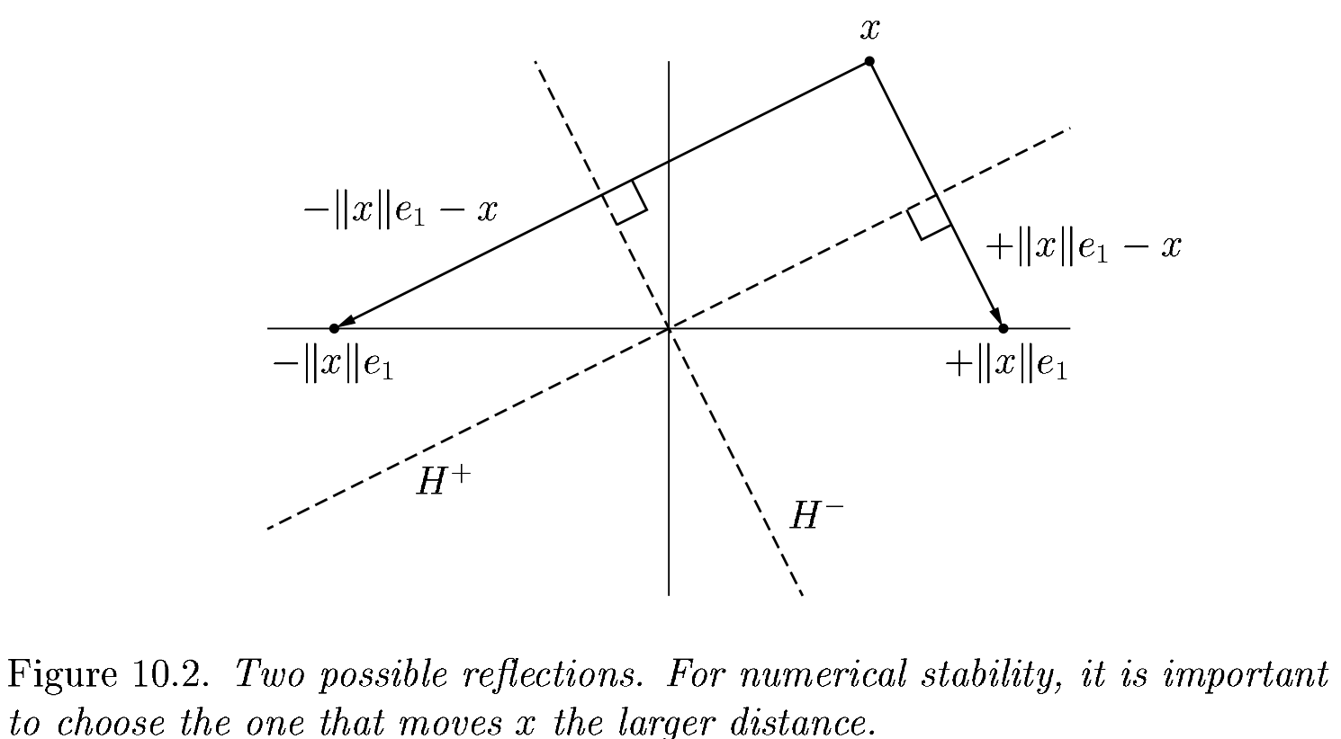
We had the lines
    v = copy(R[j:end, j])
    v[1] -= norm(v)
    v = normalize(v)
What happens when R is already upper triangular?
An improved algorithm
function qr_householder(A)
    m, n = size(A)
    R = copy(A)
    V = [] # list of reflectors
    for j in 1:n
        v = copy(R[j:end, j])
        v[1] += sign(v[1]) * norm(v) # <---
        v = normalize(v)
        R[j:end,j:end] -= 2 * v * v' * R[j:end,j:end]
        push!(V, v)
    end
    V, R
end
qr_householder (generic function with 1 method)
A = [2 -1; -1 2] * 1e-10
V, R = qr_householder(A)
tau = [2*v[1]^2 for v in V]
@show tau
V1 = [v ./ v[1] for v in V]
@show V1
R
tau = [1.894427190999916, 2.0]
V1 = [[1.0, -0.2360679774997897], [1.0]]
2×2 Matrix{Float64}:
 -2.23607e-10   1.78885e-10
 -1.29247e-26  -1.34164e-10
Householder is backward stable
m = 40
x = LinRange(-1, 1, m)
A = vander(x, m)
V, R = qr_householder(A)
Q = reflectors_to_dense(V)
@show norm(Q' * Q - I)
@show norm(Q * R - A);
norm(Q' * Q - I) = 5.949301496893686e-15
norm(Q * R - A) = 1.2090264267288813e-14
A = [1 0; 0 1.]
V, R = qr_householder(A)
qr(A)
LinearAlgebra.QRCompactWY{Float64, Matrix{Float64}}
Q factor:
2×2 LinearAlgebra.QRCompactWYQ{Float64, Matrix{Float64}}:
 1.0  0.0
 0.0  1.0
R factor:
2×2 Matrix{Float64}:
 1.0  0.0
 0.0  1.0
Orthogonality is preserved
x = LinRange(-1, 1, 20)
A = vander(x)
Q, _ = gram_schmidt_classical(A)
v = A[:,end]
@show norm(v)
scatter(abs.(Q[:,1:end-1]' * v), yscale=:log10, title="Classical Gram-Schmidt")
norm(v) = 1.4245900685395503

Q = reflectors_to_dense(qr_householder(A)[1])
scatter(abs.(Q[:,1:end-1]' * v), yscale=:log10, title="Householder QR")
