2023-02-22 QR Stability
Contents
2023-02-22 QR Stability#
Last time#
Gram-Schmidt process
QR factorization
Today#
Stability and ill conditioning
Intro to performance modeling
Classical vs Modified Gram-Schmidt
Right vs left-looking algorithms
using LinearAlgebra
using Plots
using Polynomials
default(linewidth=4, legendfontsize=12)

function vander(x, k=nothing)
    if isnothing(k)
        k = length(x)
    end
    m = length(x)
    V = ones(m, k)
    for j in 2:k
        V[:, j] = V[:, j-1] .* x
    end
    V
end
vander (generic function with 2 methods)
Gram-Schmidt orthogonalization#
Suppose we’re given some vectors and want to find an orthogonal basis for their span.
A naive algorithm#
function gram_schmidt_naive(A)
    m, n = size(A)
    Q = zeros(m, n)
    R = zeros(n, n)
    for j in 1:n
        v = A[:,j]
        for k in 1:j-1
            r = Q[:,k]' * v
            v -= Q[:,k] * r
            R[k,j] = r
        end
        R[j,j] = norm(v)
        Q[:,j] = v / R[j,j]
    end
    Q, R
end
gram_schmidt_naive (generic function with 1 method)
x = LinRange(-1, 1, 20)
A = vander(x, 20)
Q, R = gram_schmidt_naive(A)
@show norm(Q' * Q - I)
@show norm(Q * R - A);
norm(Q' * Q - I) = 1.073721107832196e-8
norm(Q * R - A) = 8.268821431611631e-16
What do orthogonal polynomials look like?#
x = LinRange(-1, 1, 50)
A = vander(x, 6)
Q, R = gram_schmidt_naive(A)
plot(x, Q)
What happens if we use more than 50 values of \(x\)? Is there a continuous limit?
Solving equations using \(QR = A\)#
If \(A x = b\) then \(Rx = Q^T b\). (Why is it easy to solve with \(R\)?)
x1 = [-0.9, 0.1, 0.5, 0.8] # points where we know values
y1 = [1, 2.4, -0.2, 1.3]
scatter(x1, y1)
A = vander(x1, 3)
Q, R = gram_schmidt_naive(A)
p = R \ (Q' * y1)
p = A \ y1
plot!(x, vander(x, 3) * p)
How accurate is it?#
m = 10
x = LinRange(-1, 1, m)
A = vander(x)
Q, R = gram_schmidt_naive(A)
@show norm(Q' * Q - I)
@show norm(Q * R - A)
norm(Q' * Q - I) = 2.2794113434933815e-13
norm(Q * R - A) = 3.6437542961698333e-16
3.6437542961698333e-16
A variant with more parallelism#
function gram_schmidt_classical(A)
    m, n = size(A)
    Q = zeros(m, n)
    R = zeros(n, n)
    for j in 1:n
        v = A[:,j]
        R[1:j-1,j] = Q[:,1:j-1]' * v
        v -= Q[:,1:j-1] * R[1:j-1,j]
        R[j,j] = norm(v)
        Q[:,j] = v / R[j,j]
    end
    Q, R
end
gram_schmidt_classical (generic function with 1 method)
norm([0 1; 1 0])
1.4142135623730951
m = 20
x = LinRange(-1, 1, m)
A = vander(x, m)
Q, R = gram_schmidt_classical(A)
@show norm(Q' * Q - I)
@show norm(Q * R - A)
norm(Q' * Q - I) = 1.4985231287367549
norm(Q * R - A) = 7.350692433565389e-16
7.350692433565389e-16
Why does order of operations matter?#
is not exact in finite arithmetic.
We can look at the size of what’s left over#
We project out the components of our vectors in the directions of each \(q_j\).
x = LinRange(-1, 1, 23)
A = vander(x)
Q, R = gram_schmidt_classical(A)
scatter(diag(R), yscale=:log10)
The next vector is almost linearly dependent#
x = LinRange(-1, 1, 20)
A = vander(x)
Q, _ = gram_schmidt_classical(A)
#Q, _ = qr(A)
v = A[:,end]
@show norm(v)
scatter(abs.(Q[:,1:end-1]' * v), yscale=:log10)
norm(v) = 1.4245900685395503
Cost of Gram-Schmidt?#
We’ll count flops (addition, multiplication, division*)
Inner product \(\sum_{i=1}^m x_i y_i\)?
Vector “axpy”: \(y_i = a x_i + y_i\), \(i \in [1, 2, \dotsc, m]\).
Look at the inner loop:
for k in 1:j-1
    r = Q[:,k]' * v
    v -= Q[:,k] * r
    R[k,j] = r
end

Counting flops is a bad model#
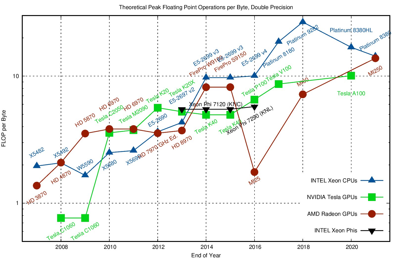
We load a single entry (8 bytes) and do 2 flops (add + multiply). That’s an arithmetic intensity of 0.25 flops/byte.
Current hardware can do about 10 flops per byte, so our best algorithms will run at about 2% efficiency.
Need to focus on memory bandwidth, not flops.
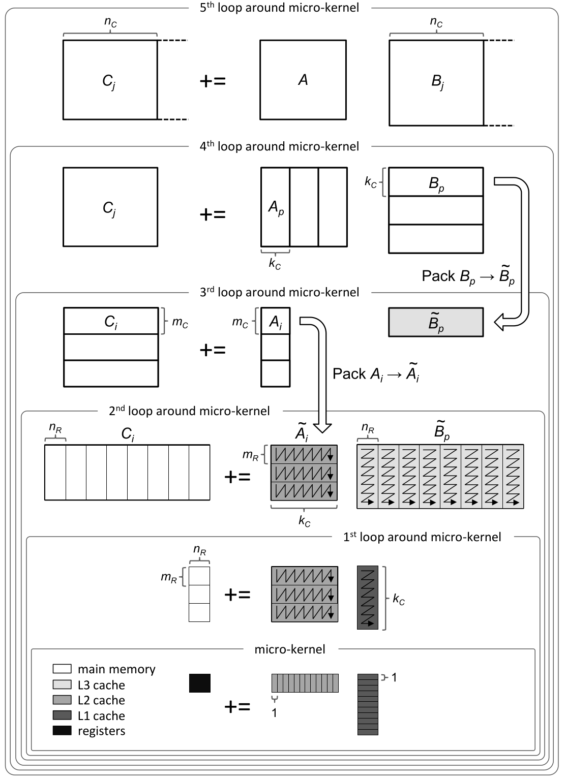
Dense matrix-matrix mulitply#

Inherent data dependencies#
Right-looking modified Gram-Schmidt#
function gram_schmidt_modified(A)
    m, n = size(A)
    Q = copy(A)
    R = zeros(n, n)
    for j in 1:n
        R[j,j] = norm(Q[:,j])
        Q[:,j] /= R[j,j]
        R[j,j+1:end] = Q[:,j]'*Q[:,j+1:end]
        Q[:,j+1:end] -= Q[:,j]*R[j,j+1:end]'
    end
    Q, R
end
gram_schmidt_modified (generic function with 1 method)
m = 20
x = LinRange(-1, 1, m)
A = vander(x, m)
Q, R = gram_schmidt_modified(A)
@show norm(Q' * Q - I)
@show norm(Q * R - A)
norm(Q' * Q - I) = 8.486718528276085e-9
norm(Q * R - A) = 8.709998074379606e-16
8.709998074379606e-16
Classical versus modified?#
Classical
Really unstable, orthogonality error of size \(1 \gg \epsilon_{\text{machine}}\)
Don’t need to know all the vectors in advance
Modified
Needs to be right-looking for efficiency
Less unstable, but orthogonality error \(10^{-9} \gg \epsilon_{\text{machine}}\)
m = 10
x = LinRange(-1, 1, m)
A = vander(x, m)
Q, R = qr(A)
@show norm(Q' * Q - I)
norm(Q' * Q - I) = 2.2760345477368898e-15
2.2760345477368898e-15
