
2025-09-29 QR Retrospective#
Last time#
Right vs left-looking algorithms
Elementary reflectors
Householder QR
Today#
Householder fix
Comparison of interfaces
Profiling
Cholesky QR
using LinearAlgebra
using Plots
default(linewidth=4, legendfontsize=12)

function vander(x, k=nothing)
    if isnothing(k)
        k = length(x)
    end
    m = length(x)
    V = ones(m, k)
    for j in 2:k
        V[:, j] = V[:, j-1] .* x
    end
    V
end

function gram_schmidt_classical(A)
    m, n = size(A)
    Q = zeros(m, n)
    R = zeros(n, n)
    for j in 1:n
        v = A[:,j]
        R[1:j-1,j] = Q[:,1:j-1]' * v
        v -= Q[:,1:j-1] * R[1:j-1,j]
        R[j,j] = norm(v)
        Q[:,j] = v / R[j,j]
    end
    Q, R
end
gram_schmidt_classical (generic function with 1 method)
Householder QR#
Gram-Schmidt constructed a triangular matrix \(R\) to orthogonalize \(A\) into \(Q\). Each step was a projector, which is a rank-deficient operation. Householder uses orthogonal transformations (reflectors) to triangularize.
The structure of the algorithm is
Constructing the \(Q_j\)#
Each of our \(Q_j\) will have the form
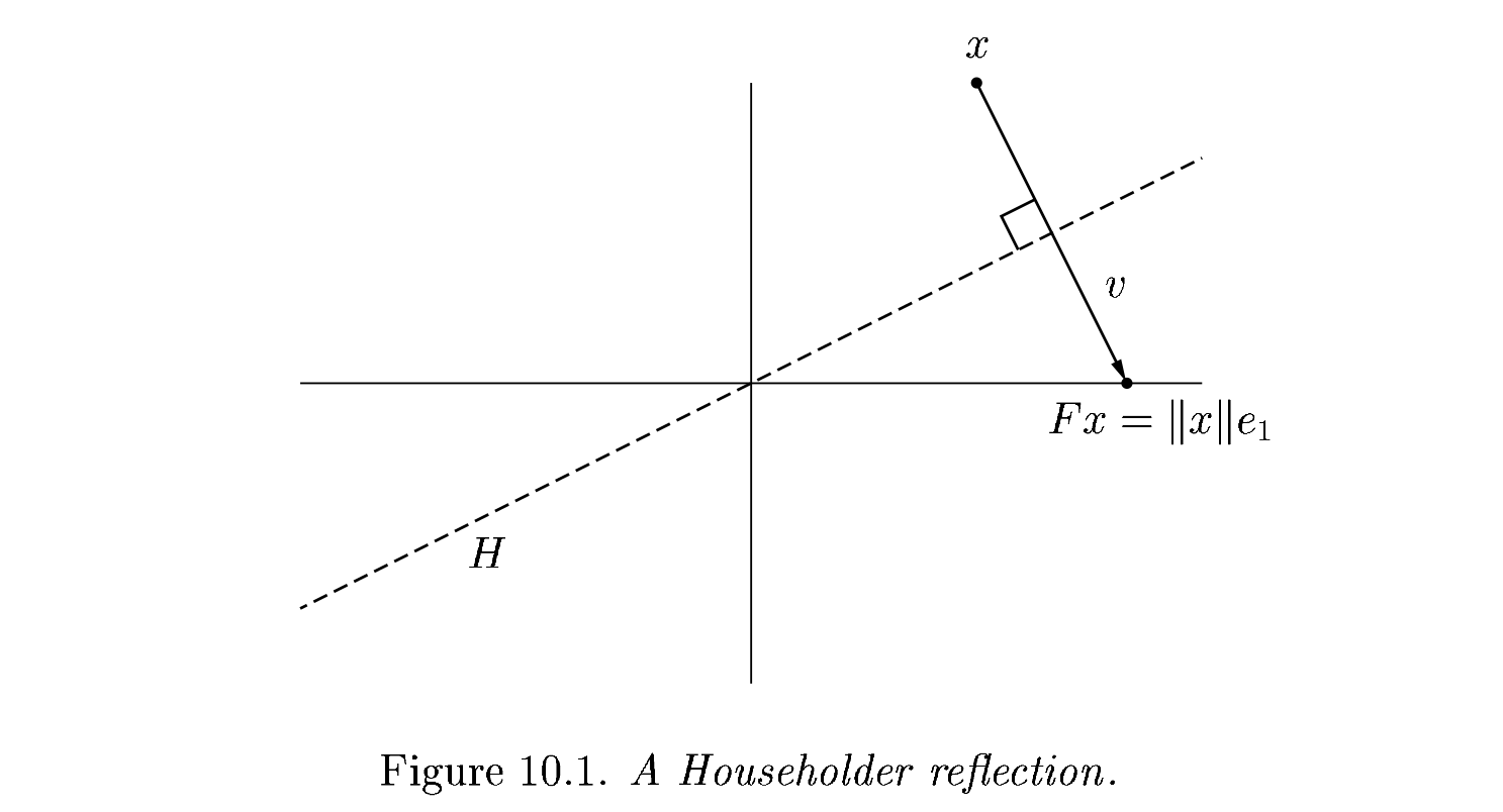
The reflection, as depicted above by Trefethen and Bau (1999) can be written \(F = I - 2 \frac{v v^T}{v^T v}\).
Adventures in reflection#
A = rand(4, 4); A += A'
v = copy(A[:,1])
v[1] -= norm(v)
v = normalize(v)
F = I - 2 * v * v'
B = F * A
4×4 Matrix{Float64}:
 2.00074       2.19872    1.91185    2.2909
 1.54919e-16   0.242686  -0.808393  -0.281889
 9.41728e-17   0.434702   0.71182    0.987804
 1.88833e-16  -0.647386  -0.62522   -0.158602
v = copy(B[2:end, 2])
v[1] -= norm(v); v = normalize(v)
F = I - 2 * v * v'
B[2:end, 2:end] = F * B[2:end, 2:end]
B
4×4 Matrix{Float64}:
 2.00074       2.19872       1.91185   2.2909
 1.54919e-16   0.816682      0.634276  0.567744
 9.41728e-17   1.11022e-16  -0.380749  0.344356
 1.88833e-16  -1.66533e-16   1.0019    0.799661
An algorithm#
function qr_householder_naive(A)
    m, n = size(A)
    R = copy(A)
    V = [] # list of reflectors
    for j in 1:n
        v = copy(R[j:end, j])
        v[1] -= norm(v)
        v = normalize(v)
        R[j:end,j:end] -= 2 * v * (v' * R[j:end,j:end])
        push!(V, v)
    end
    V, R
end
qr_householder_naive (generic function with 1 method)
m = 4
x = LinRange(-1, 1, m)
A = vander(x, m)
V, R = qr_householder_naive(A)
_, R_ = qr(A)
R_
4×4 Matrix{Float64}:
 -2.0  0.0      -1.11111      0.0
  0.0  1.49071   1.38778e-17  1.3582
  0.0  0.0       0.888889     9.71445e-17
  0.0  0.0       0.0          0.397523
How to interpret \(V\) as \(Q\)?#
function reflectors_mult(V, x)
    y = copy(x)
    for v in reverse(V)
        n = length(v) - 1
        y[end-n:end] -= 2 * v * (v' * y[end-n:end])
    end
    y
end

function reflectors_to_dense(V)
    m = length(V[1])
    Q = diagm(ones(m))
    for j in 1:m
        Q[:,j] = reflectors_mult(V, Q[:,j])
    end
    Q
end
reflectors_to_dense (generic function with 1 method)
m = 20
x = LinRange(-1, 1, m)
A = vander(x, m)
V, R = qr_householder_naive(A)
Q = reflectors_to_dense(V)
@show norm(Q' * Q - I)
@show norm(Q * R - A);
norm(Q' * Q - I) = 3.7994490775439526e-15
norm(Q * R - A) = 7.562760794606217e-15
Great, but we can still break it#
A = [0 2; 1e-2 1.]
V, R = qr_householder(A)
#Q, R = qr(A)
R
2×2 Matrix{Float64}:
  0.01          1.0
 -1.73472e-18  -2.0
We had the lines
    v = copy(R[j:end, j])
    v[1] -= norm(v)
    v = normalize(v)
What happens when R is already upper triangular?
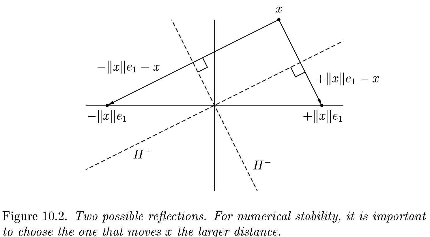
An improved algorithm#
function qr_householder(A)
    m, n = size(A)
    R = copy(A)
    V = [] # list of reflectors
    for j in 1:n
        v = copy(R[j:end, j])
        #v[1] += sign(v[1]) * norm(v) # <---
        v[1] += (v[1] > 0 ? 1 : -1) * norm(v)
        v = normalize(v)
        R[j:end,j:end] -= 2 * v * v' * R[j:end,j:end]
        push!(V, v)
    end
    V, R
end
qr_householder (generic function with 1 method)
A = [2 -1; -1 2] * 1e-10
V, R = qr_householder(A)
tau = [2*v[1]^2 for v in V]
@show tau
V1 = [v ./ v[1] for v in V]
@show V1
R
tau = [1.894427190999916, 2.0]
V1 = [[1.0, -0.2360679774997897], [1.0]]
2×2 Matrix{Float64}:
 -2.23607e-10   1.78885e-10
 -1.29247e-26  -1.34164e-10
Householder is backward stable#
m = 40
x = LinRange(-1, 1, m)
A = vander(x, m)
V, R = qr_householder(A)
Q = reflectors_to_dense(V)
@show norm(Q' * Q - I)
@show norm(Q * R - A);
norm(Q' * Q - I) = 5.949301496893686e-15
norm(Q * R - A) = 1.2090264267288813e-14
A = [1 0; 0 1.]
V, R = qr_householder(A)
#qr(A)
(Any[[1.0, 0.0], [1.0]], [-1.0 0.0; 0.0 -1.0])
Orthogonality is preserved#
x = LinRange(-1, 1, 20)
A = vander(x)
Q, _ = gram_schmidt_classical(A)
v = A[:,end]
@show norm(v)
scatter(abs.(Q[:,1:end-1]' * v), yscale=:log10, title="Classical Gram-Schmidt")
norm(v) = 1.4245900685395503
Q = reflectors_to_dense(qr_householder(A)[1])
scatter(abs.(Q[:,1:end-1]' * v), yscale=:log10, title="Householder QR")
Composition of reflectors#
This turns applying reflectors from a sequence of vector operations to a sequence of (smallish) matrix operations. It’s the key to high performance and the native format (QRCompactWY) returned by Julia qr().
Q, R = qr(A)
LinearAlgebra.QRCompactWY{Float64, Matrix{Float64}, Matrix{Float64}}
Q factor: 20×20 LinearAlgebra.QRCompactWYQ{Float64, Matrix{Float64}, Matrix{Float64}}
R factor:
20×20 Matrix{Float64}:
 -4.47214  0.0      -1.64763       0.0          …  -0.514468      2.22045e-16
  0.0      2.71448   1.11022e-16   1.79412         -2.498e-16     0.823354
  0.0      0.0      -1.46813       5.55112e-17     -0.944961     -2.23779e-16
  0.0      0.0       0.0          -0.774796         3.83808e-17  -0.913056
  0.0      0.0       0.0           0.0              0.797217     -4.06264e-16
  0.0      0.0       0.0           0.0          …  -3.59496e-16   0.637796
  0.0      0.0       0.0           0.0             -0.455484     -1.3936e-15
  0.0      0.0       0.0           0.0              4.40958e-16  -0.313652
  0.0      0.0       0.0           0.0             -0.183132      1.64685e-15
  0.0      0.0       0.0           0.0              4.82253e-16   0.109523
  0.0      0.0       0.0           0.0          …   0.0510878     5.9848e-16
  0.0      0.0       0.0           0.0             -2.68709e-15   0.0264553
  0.0      0.0       0.0           0.0             -0.0094344    -2.94383e-15
  0.0      0.0       0.0           0.0              2.08514e-15   0.00417208
  0.0      0.0       0.0           0.0              0.0010525    -2.24994e-15
  0.0      0.0       0.0           0.0          …  -1.64363e-15  -0.000385264
  0.0      0.0       0.0           0.0             -5.9057e-5     7.69025e-16
  0.0      0.0       0.0           0.0              1.76642e-16  -1.66202e-5
  0.0      0.0       0.0           0.0             -1.04299e-6   -1.68771e-16
  0.0      0.0       0.0           0.0              0.0           1.71467e-7
This works even for very nonsquare matrices#
A = rand(1000000, 5)
Q, R = qr(A)
@show size(Q)
@show norm(Q*R - A)
R
size(Q) = (1000000, 1000000)
norm(Q * R - A) = 3.059842369178539e-12
5×5 Matrix{Float64}:
 -577.004  -433.339  -433.146  -433.187  -433.032
    0.0     381.804   163.137   163.734   163.39
    0.0       0.0     345.012   103.551   103.128
    0.0       0.0       0.0    -329.306   -75.7609
    0.0       0.0       0.0       0.0    -320.388
This is known as a “full” (or “complete”) QR factorization, in contrast to a reduced QR factorization in which \(Q\) has the same shape as \(A\).
How much memory does \(Q\) use?
Compare to numpy.linalg.qr#
Need to decide up-front whether you want full or reduced QR.
Full QR is expensive to represent.
Cholesky QR#
so we should be able to use \(L L^T = A^T A\) and then \(Q = A L^{-T}\).
function qr_chol(A)
    R = cholesky(A' * A).U
    Q = A / R
    Q, R
end

A = rand(10,4)
Q, R = qr_chol(A)
@show norm(Q' * Q - I)
@show norm(Q * R - A)
norm(Q' * Q - I) = 2.2107277380745723e-15
norm(Q * R - A) = 4.3488656054059265e-16
4.3488656054059265e-16
x = LinRange(-1, 1, 20)
A = vander(x)
Q, R = qr_chol(A)
@show norm(Q' * Q - I)
@show norm(Q * R - A);
norm(Q' * Q - I) = 0.1749736012761826
norm(Q * R - A) = 6.520306397146206e-16
Can we fix this?#
Note that the product of two triangular matrices is triangular.
R = triu(rand(5,5))
R * R
5×5 Matrix{Float64}:
 0.97317  0.166549  0.886643   0.790819  1.41736
 0.0      0.62048   0.559597   1.00648   1.62617
 0.0      0.0       0.0145787  0.449376  0.587352
 0.0      0.0       0.0        0.940909  1.08426
 0.0      0.0       0.0        0.0       0.122084
function qr_chol2(A)
    Q, R = qr_chol(A)
    Q, R1 = qr_chol(Q)
    Q, R1 * R
end

x = LinRange(-1, 1, 20)
A = vander(x)
Q, R = qr_chol2(A)
@show norm(Q' * Q - I)
@show norm(Q * R - A);
norm(Q' * Q - I) = 1.3276319786294278e-15
norm(Q * R - A) = 1.0894860257129427e-15
How fast are these methods?#
m, n = 5000, 4000
A = randn(m, n)

@time qr(A);
1.070449 seconds (9 allocations: 154.787 MiB, 0.06% gc time)
A = randn(m, n)
@time qr_chol(A);
1.201750 seconds (10 allocations: 396.738 MiB, 17.43% gc time)
Profiling#
using ProfileSVG

#@profview qr(A)
@profview qr_chol(A)
Krylov subspaces#
Suppose we wish to solve
but only have the ability to apply the action of the \(A\) (we do not have access to its entries). A general approach is to work with approximations in a Krylov subspace, which has the form
This matrix is horribly ill-conditioned and cannot stably be computed as written. Instead, we seek an orthogonal basis \(Q_n\) that spans the same space as \(K_n\). We could write this as a factorization
where the first column \(q_1 = b / \lVert b \rVert\). The \(R_n\) is unnecessary and hopelessly ill-conditioned, so a slightly different procedure is used.
Arnoldi iteration#
The Arnoldi iteration applies orthogonal similarity transformations to reduce \(A\) to Hessenberg form, starting from a vector \(q_1 = b/\lVert b \rVert\),
Let’s multiply on the right by \(Q\) and examine the first \(n\) columns,
where \(H_n\) is an \((n+1) \times n\) Hessenberg matrix.
GMRES#
GMRES (Generalized Minimum Residual) minimizes
Notes#
The solution \(x_n\) constructed by GMRES at iteration \(n\) is not explicitly available. If a solution is needed, it must be constructed by solving the \((n+1)\times n\) least squares problem and forming the solution as a linear combination of the \(n\) vectors \(Q_n\). The leading cost is \(2mn\) where \(m \gg n\).
The residual vector \(r_n = A x_n - b\) is not explicitly available in GMRES. To compute it, first build the solution \(x_n = Q_n y_n\).
GMRES minimizes the 2-norm of the residual \(\lVert r_n \rVert\) which is equivalent to the \(A^* A\) norm of the error \(\lVert x_n - x_* \rVert_{A^* A}\).
More notes on GMRES#
GMRES needs to store the full \(Q_n\), which is unaffordable for large \(n\) (many iterations). The standard solution is to choose a “restart” \(k\) and to discard \(Q_n\) and start over with an initial guess \(x_k\) after each \(k\) iterations. This algorithm is called GMRES(k). PETSc’s default solver is GMRES(30) and the restart can be controlled using the run-time option
-ksp_gmres_restart.Most implementations of GMRES use classical Gram-Schmidt because it is much faster in parallel (one reduction per iteration instead of \(n\) reductions per iteration). The PETSc option
-ksp_gmres_modifiedgramschmidtcan be used when you suspect that classical Gram-Schmidt may be causing instability.There is a very similar (and older) algorithm called GCR that maintains \(x_n\) and \(r_n\). This is useful, for example, if a convergence tolerance needs to inspect individual entries. GCR requires \(2n\) vectors instead of \(n\) vectors, and can tolerate a nonlinear preconditioner. FGMRES is a newer algorithm with similar properties to GCR.