
2025-09-05 Rootfinding#
Last time#
Forward and backward error
Forward and backward stability
Computing volume of a polygon
Goal-setting and activity
Discussion of errors
Today#
Rootfinding as a modeling tool
Use Roots.jl to solve
Introduce Bisection
Convergence classes
Intro to Newton methods
using Plots
default(linewidth=4)
Rootfinding#
Given \(f(x)\), find \(x\) such that \(f(x) = 0\).
We’ll work with scalars (\(f\) and \(x\) are just numbers) for now, and revisit later when they vector-valued.
Change inputs to outputs#
\(f(x; b) = x^2 - b\)
\(x(b) = \sqrt{b}\)
\(f(x; b) = \tan x - b\)
\(x(b) = \arctan b\)
\(f(x) = \cos x + x - b\)
\(x(b) = ?\)
We aren’t given \(f(x)\), but rather an algorithm f(x) that approximates it.
Sometimes we get extra information, like
fp(x)that approximates \(f'(x)\)If we have source code for
f(x), maybe it can be transformed “automatically”
Nesting matryoshka dolls of rootfinding#
I have a function (pressure, temperature) \(\mapsto\) (density, energy)
I need (density, energy) \(\mapsto\) (pressure, temperature)
I know what condition is satisfied across waves, but not the state on each side.
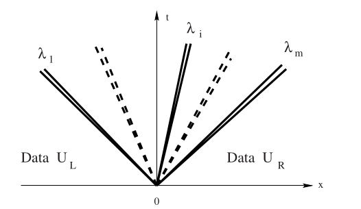
Toro (2009)
Given a proposed state, I can measure how much (mass, momentum, energy) is not conserved.
Find the solution that conserves exactly
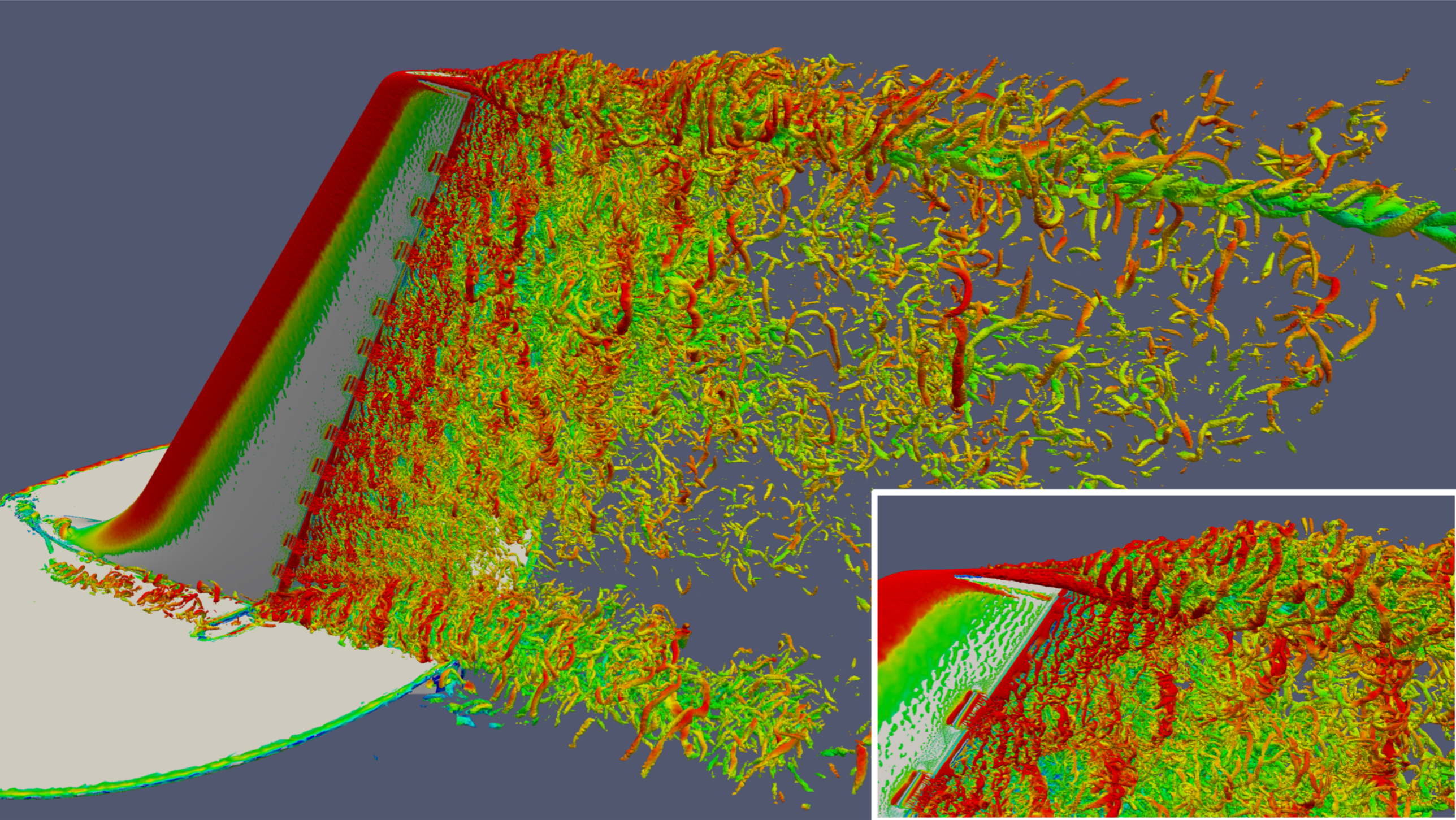
I can compute lift given speed and angle of attack
How much can the plane lift?
How much can it lift on a short runway?
Discuss: rootfinding and inverse problems#
Inverse kinematics for robotics
(statics) how much does each joint an robotic arm need to move to grasp an object
(with momentum) fastest way to get there (motors and arms have finite strength)
similar for virtual reality
Infer a light source (or lenses/mirrors) from an iluminated scene
Imaging
radiologist seeing an x-ray is mentally inferring 3D geometry from 2D image
computed tomography (CT) reconstructs 3D model from multiple 2D x-ray images
seismology infers subsurface/deep earth structure from seismograpms
Example: Queueing#
In a simple queueing model, there is an arrival rate and a departure (serving) rate. While waiting in the queue, there is a probability of “dropping out”. The length of the queue in this model is
One model for the waiting time (where these rates are taken from exponential distributions) is
wait(arrival, departure) = log(arrival / departure) / departure

plot(d -> wait(1, d), xlims=(.1, 1), xlabel="departure", ylabel="wait")
Departure rate given wait#
Easy to measure wait
I have a limited tolerance for waiting
my_wait = 0.8
plot([d -> wait(1, d) - my_wait, d -> 0], xlims=(.1, 1), xlabel="departure", ylabel="wait")
#import Pkg; Pkg.add("Roots")
using Roots
d0 = find_zero(d -> wait(1, d) - my_wait, 1)
plot([d -> wait(1, d) - my_wait, d -> 0], xlims=(.1, 1), xlabel="departure", ylabel="wait")
scatter!([d0], [0], marker=:circle, color=:black, title="d0 = $d0")
Example: Nonlinear Elasticity#
Strain-energy formulation#
where \(I_1 = \lambda_1^2 + \lambda_2^2 + \lambda_3^3\) and \(J = \lambda_1 \lambda_2 \lambda_3\) are invariants defined in terms of the principle stretches \(\lambda_i\).
Uniaxial extension#
In the experiment, we would like to know the stress as a function of the stretch \(\lambda_1\). We don’t know \(J\), and will have to determine it by solving an equation.
How much does the volume change?#
Using symmetries of uniaxial extension, we can write an equation \(f(\lambda, J) = 0\) that must be satisfied. We’ll need to solve a rootfinding problem to compute \(J(\lambda)\).
function f(lambda, J)
    C_1 = 1.5e6
    D_1 = 1e8
    D_1 * J^(8/3) - D_1 * J^(5/3) + C_1 / (3*lambda) * J - C_1 * lambda^2/3
end
plot(J -> f(4, J), xlims=(0.1, 3), xlabel="J", ylabel="f(J)")
find_J(lambda) = find_zero(J -> f(lambda, J), 1)
plot(find_J, xlims=(0.1, 5), xlabel="lambda", ylabel="J")
An algorithm: Bisection#
Bisection is a rootfinding technique that starts with an interval \([a,b]\) containing a root and does not require derivatives. Suppose \(f\) is continuous. What is a sufficient condition for \(f\) to have a root on \([a,b]\)?
hasroot(f, a, b) = f(a) * f(b) < 0

f(x) = cos(x) - x
plot(f)
Bisection#
function bisect(f, a, b, tol)
    mid = (a + b) / 2
    if abs(b - a) < tol
        return mid
    elseif hasroot(f, a, mid)
        return bisect(f, a, mid, tol)
    else
        return bisect(f, mid, b, tol)
    end
end

x0 = bisect(f, -1, 3, 1e-5)
x0, f(x0)
(0.7390861511230469, -1.7035832658995886e-6)
How fast does it converge?#
function bisect_hist(f, a, b, tol)
    mid = (a + b) / 2
    if abs(b - a) < tol
        return [mid]
    elseif hasroot(f, a, mid)
        return prepend!(bisect_hist(f, a, mid, tol), [mid])
    else
        return prepend!(bisect_hist(f, mid, b, tol), [mid])
    end
end
bisect_hist (generic function with 1 method)
bisect_hist(f, -1, 3, 1e-4)
17-element Vector{Float64}:
 1.0
 0.0
 0.5
 0.75
 0.625
 0.6875
 0.71875
 0.734375
 0.7421875
 0.73828125
 0.740234375
 0.7392578125
 0.73876953125
 0.739013671875
 0.7391357421875
 0.73907470703125
 0.739105224609375
Iterative bisection#
Data structures often optimized for appending rather than prepending.
Bounds stack space
f(x) = cos(x) - x
hasroot(f, a, b) = f(a) * f(b) < 0
function bisect_iter(f, a, b, tol)
    hist = Float64[]
    while abs(b - a) > tol
        mid = (a + b) / 2
        push!(hist, mid)
        if hasroot(f, a, mid)
            b = mid
        else
            a = mid
        end
    end
    hist
end
bisect_iter (generic function with 1 method)
length(bisect_iter(f, -1, 3, 1e-20))
56
Let’s plot the error#
where \(r\) is the true root, \(f(r) = 0\).
hist = bisect_iter(f, -1, 3, 1e-10)
r = hist[end] # What are we trusting?
hist = hist[1:end-1]
scatter( abs.(hist .- r), yscale=:log10)
ks = 1:length(hist)
plot!(ks, 4 * (.5 .^ ks))
Evidently the error \(e_k = x_k - x_*\) after \(k\) bisections satisfies the bound
Convergence classes#
A convergent rootfinding algorithm produces a sequence of approximations \(x_k\) such that
ρ = 0.8
errors = [1.]
for i in 1:30
    next_e = errors[end] * ρ
    push!(errors, next_e)
end
plot(errors, yscale=:log10, ylims=(1e-10, 1))
e = hist .- r
scatter(abs.(errors[2:end] ./ errors[1:end-1]), ylims=(0,1))
Bisection: A = q-linearly convergent, B = r-linearly convergent, C = neither#
Remarks on bisection#
Specifying an interval is often inconvenient
An interval in which the function changes sign guarantees convergence (robustness)
No derivative information is required
If bisection works for \(f(x)\), then it works and gives the same accuracy for \(f(x) \sigma(x)\) where \(\sigma(x) > 0\).
Roots of even degree are problematic
A bound on the solution error is directly available
The convergence rate is modest – one iteration per bit of accuracy
For you#
Share an equation that is useful for one task, but requires rootfinding for another task.
OR: explain a system in which one stakeholder has the natural inputs, but a different stakeholder only knows outputs.
Please collaborate.